Solar panels for homes are rooftop or ground-mounted photovoltaic systems that convert sunlight into electricity for residential use. Understanding the costs, potential savings, and payback timeframes involves examining up-front hardware and installation expenses, ongoing operating factors, and how household electricity consumption patterns interact with local electricity pricing or compensation schemes. A clear view of these elements helps homeowners and analysts compare scenarios where on-site generation offsets grid purchases or charges batteries for later use. This discussion focuses on the practical dimensions of cost and value without promising specific financial results.
Key considerations include system size in kilowatts (kW), panel and inverter types, mounting and labor, permitting, and potential costs for upgrades such as roof reinforcement or electrical panel work. Ongoing variables that affect long-term value may include panel degradation, inverter replacement, local weather patterns, and policy frameworks for crediting exported energy. Calculating potential savings typically requires comparing projected on-site generation to historical household consumption and local retail electricity rates or export compensation approaches. Estimates should be treated as scenario-based rather than guaranteed outcomes.
Comparative analysis of these examples often begins with installation cost ranges expressed per watt or per kilowatt and scaled by system size. Typical residential systems may range widely depending on region, labor rates, and component levels of quality or efficiency. For instance, equipment quality can affect both initial cost and expected energy yield per square metre. When assessing scenarios, modelled annual energy production and expected degradation rates are primary inputs; these feed into cash-flow estimates that produce payback ranges. All numerical inputs should be treated as illustrative and adjusted to reflect local conditions.
Estimating potential savings requires combining projected generation with household consumption patterns and the structure of local electricity tariffs. If exported energy receives credit at retail rates, avoided costs per kilowatt-hour may be higher than when exports are compensated at lower rates. Time-of-use tariffs can change the value of on-site generation and storage: shifting consumption to midday solar production may increase value where on-peak rates are higher. Sensitivity analysis commonly varies electricity price escalation, panel output, and system availability to illustrate plausible payback windows.
System components influence both cost and long-term performance. Panels, inverters, mounting hardware, wiring, and metering each contribute to initial expense and have different lifespans and maintenance needs. Panels typically show gradual performance decline; inverters often require replacement sooner than modules. Battery systems add capital and may require specific maintenance or replacement cycles depending on chemistry and cycling patterns. Factoring component lifespans into lifecycle cost modelling helps produce more realistic payback estimates and replacement timing expectations.
Non-equipment factors can shift payback timeframes significantly. Local permitting and inspection fees, interconnection rules, and the need for any roof or electrical upgrades may add to up-front cost and extend project timelines. Climate and shading influence annual energy yield; even small shading on a string can reduce overall system output unless module-level power electronics are used. Financing terms such as interest rates, loan duration, or tax and policy incentives (where applicable) can shorten or lengthen the period until net savings exceed the initial expenditure.
In summary, residential photovoltaic systems are a combination of technical, economic, and policy variables that together determine installation cost, prospective savings, and payback timeframe. Analyses typically model multiple scenarios and sensitivity ranges rather than assert a single outcome. The next sections examine practical components and considerations in more detail.
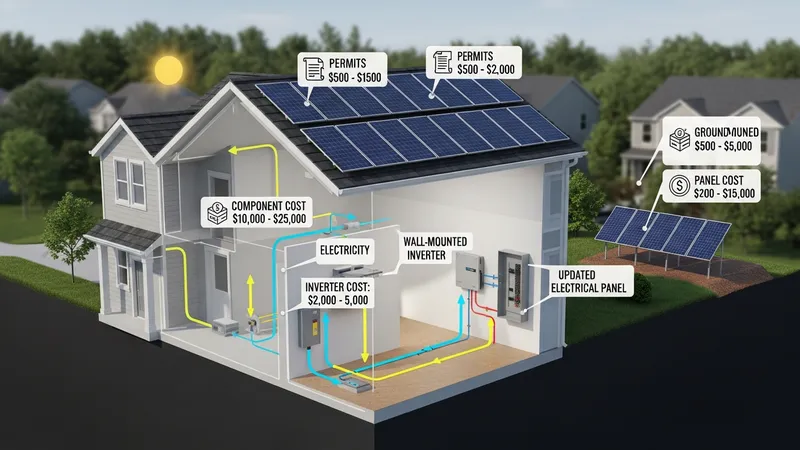
Up-front costs for residential solar systems generally break down into equipment, installation labor, permitting and inspection, and any necessary site upgrades. Equipment includes modules, inverters, racking, wiring, and sometimes batteries; installation labor covers mounting, electrical connections, and commissioning. Typical per-watt pricing often varies by region, installer overhead, and equipment choices. When performing cost estimates, it is useful to separate hard costs (hardware) from soft costs (permits, design, interconnection) and to account for potential additional costs such as structural reinforcement or electrical panel replacement. Conservative budgeting may avoid underestimating soft costs.
Component selection can influence both initial price and expected operational profile. Higher-efficiency modules can reduce roof area required for a given output but may carry a premium; string inverters are often less costly than microinverters or optimisers but may perform differently under partial shading. Battery chemistry and capacity choices affect capital cost and depth-of-discharge patterns, which in turn influence lifetime throughput. When comparing costs, it can be informative to model levelized cost of energy from the system over a multi-decade horizon while including anticipated replacements and maintenance.
Installation logistics and local regulations may add variability to total project price and timeline. Permit fees, interconnection application processes, and utility inspection requirements can contribute to soft costs and delay system operation. If roof work or conduit runs are complex, labor hours may increase. Accurate site assessments that include shade analysis, roof condition evaluation, and electrical panel checks often reduce the likelihood of unplanned expenses during installation. Including contingency allowances for unforeseen site issues is a common practice in realistic budgeting.
Detailed cost modelling typically uses scenario inputs such as system size, expected annual production, component degradation, and financing terms. Sensitivity analyses that vary electricity price inflation, system uptime, or inverter replacement timing can clarify how sensitive payback timeframes are to each factor. Presenting a range of outcomes—such as shorter and longer payback scenarios—helps set expectations and highlights which variables most strongly affect financial performance without implying certainty.
Potential savings from a residential solar system are the difference between electricity costs avoided through on-site generation and any remaining grid purchases plus system operating costs. Calculating avoided costs requires combining hourly or daily load profiles with estimated hourly generation profiles to determine self-consumption versus export. If export compensation is available, exported energy can contribute additional value. Typical methods include using historical utility bills to build a baseline consumption profile and modelling expected system output using location-specific irradiance data and tilt/azimuth configurations.
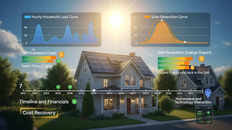
Payback timeframe is commonly expressed as the period until cumulative avoided utility expenses and any export credits offset the net project cost after financing and incentives. This timeframe may shorten when financing terms are favorable or when incentives reduce net capital outlay. Conversely, payback may extend if equipment underperforms or if electricity prices remain low. Models often use conservative assumptions for panel degradation and may include inverter replacements to reflect common maintenance cycles, which can materially shift the payback horizon in long-term projections.
Storage complicates savings calculations because batteries typically increase upfront costs while enabling time-shifting of consumption and potential demand charge reductions where relevant. The value of storage depends on tariff structures, battery round-trip efficiency, and cycling patterns. For households on time-of-use pricing, shifting consumption into midday solar production can increase avoided costs; in regions without time-of-use differentiation, the incremental economic benefit of storage may be lower and should be modelled accordingly with realistic cycling assumptions.
Scenario-based planning often presents multiple cases—base, optimistic, and conservative—each varying electricity price escalation, production, and component replacement timing. Such structured sensitivity testing highlights which inputs most influence payback estimates, such as local retail electricity prices or export compensation rules. Presenting ranges rather than single-point estimates communicates uncertainty while helping users understand trade-offs inherent in different system configurations.
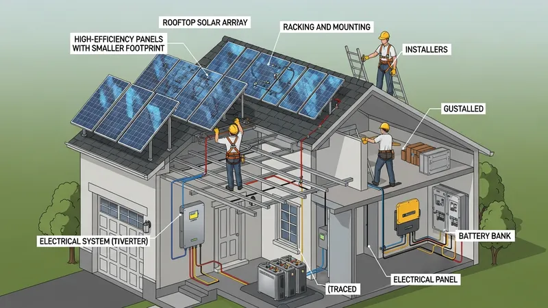
Major system components include photovoltaic modules, inverters, mounting and racking systems, wiring and breakers, metering equipment, and optional batteries. Module quality, temperature coefficients, and rated efficiency influence energy yield per installed area. Inverters convert DC to AC power and may include features such as maximum power point tracking and safety shutdown. The choice between central inverters, string inverters, microinverters, or power optimisers affects both performance under partial shading and replacement strategies. Understanding component lifespans is important when modelling lifecycle costs and expected performance.
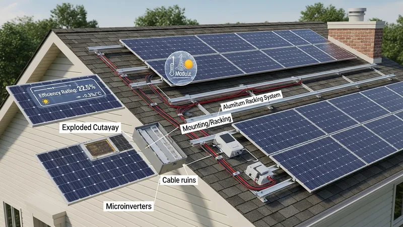
Performance factors that influence long-term yields include orientation and tilt, shading, soiling, ambient temperature, and degradation rates. Seasonal and interannual variation in sunlight can cause output to fluctuate; long-term averages are preferable for multi-year projections. Module degradation is typically gradual but should be included as a percentage decline per year in production models. Maintenance practices such as periodic cleaning and inspection of electrical connections may help maintain expected output, and these activities can be budgeted as modest ongoing operating costs.
System monitoring and diagnostics can support performance tracking and help detect underperformance or faults early. Monitoring platforms vary in granularity, with some offering module-level visibility and others reporting only whole-system output. Where available, module-level data can reveal shading or equipment issues more quickly, which may reduce long-term energy loss. Including monitoring capabilities in a project plan may increase initial cost slightly but can provide useful data for validating production against modelling assumptions.
Environmental and site-specific considerations can materially affect expected yields. Roof orientation, available unshaded area, local climate patterns, and snow or dust accumulation all influence annual generation. Structural assessments that confirm roof age and condition can prevent unexpected replacement costs shortly after installation. When modelling system performance for payback estimation, including conservative allowances for production variability helps produce more robust and realistic forecasts rather than optimistic single-point estimates.
Financing options for residential solar commonly include outright purchase, loans, leases, and power purchase agreements (PPA) where available. Each method alters initial cash outlay and the distribution of costs and benefits over time. Loan financing can spread capital cost across years and may increase nominal payback periods depending on interest rate; leases or PPAs often reduce or eliminate up-front expenditure but change the ownership of the system and the flow of savings. Comparing lifecycle outcomes across financing structures requires modelling cash flows, tax implications where relevant, and any policy incentives separately for accuracy.
Policy mechanisms such as tax credits, rebates, or export compensation frameworks can significantly influence net project economics where they exist. These instruments vary widely by jurisdiction and may change over time; therefore, sensitivity to policy shifts is prudent when estimating long-term payback. In many analyses, incentives are treated as incremental reductions in net capital cost or as line items in annual cash flows. Modellers often test scenarios with and without current incentive levels to show how dependent payback is on policy support.
Long-term ownership considerations include warranty coverage, expected maintenance, and replacement timing for components such as inverters or batteries. Manufacturer warranties for panels often cover performance for multiple decades, while inverter warranties are typically shorter; battery warranties commonly specify cycle or time limits. Accounting for end-of-life component replacement costs in multi-decade financial models affects net savings and may alter the relative attractiveness of storage additions or higher-cost components claimed to improve longevity.
When interpreting model results, it is helpful to present ranges and clarify key assumptions that drive outcomes. Sensitivity tables or tornado charts that show the relative impact of changes in electricity price, system production, or financing cost can guide non-prescriptive decisions about whether further detailed study is warranted. Continued reading of the earlier sections can help readers match assumptions to their local context and refine estimates for their specific situation.